Life Expectancy and Cost of a Life Annuity

In a neat (and mathematical) paper, in PDF format, Milevsky & Robinson discuss Life Annuities in a novel way ... well, it's novel to me. So I thought it'd be fun to (try) to explain the gist of the paper.
>With no math? Good!
Well ... some math, which you can skip over. Now, pay attention. We start with a review of cumulative probability distributions for, say, life expectancy: (See this for more on cumulative distributions.)
We suppose:

Our age is n.
We want to know the probability of dying before x years have passed
meaning: before we're n+x years old.
Consider a cumulative distribution, y = F(x), as in Fig. 1, where we pick an x-value and the y-value gives the fraction of the n-year-old population who will die within x years.
Of course, this distribution will depend not only upon x but also upon our current age, n ... so we should write y = F(n,x).
The fraction of this n-year-old population who will die somewhere between x and x+Δx years is:
the fraction who will die before x+Δx years less the fraction who will die before before x years, namely F(x+Δx)-F(x)

Fig. 1

Fig. 2 If we call the slope of the cumulative distribution f(x), then we see
(from Fig. 1) that (for small Δx)
{F(x+Δx) - F(x)}/Δx = f(x)
This guy, f(x), is called the Density Distribution. This is illustrated in Fig. 2.
>You forgot to say F(n,x) and f(n,x).
Yes. We'll assume the dependence upon n and, when necessary, I'll stick it in. Okay? In Fig. 2 is a picture of a typical cumulative distribution F(x) and
its slope f(x). In fact, for this particular picture, f(x) has the form K xⁿ e^-x.

In order to be a valid density distribution the probability of living less than an infinite number of years must be "1".
>It's 100% certain you'll die within an infinite number of years, right?
Right, and that means that the total area under the curve y = f(x) must be "1" and that means that
K = 1, but since (surprise!)
Γ(n+1) = is called the Gamma function and has the value Γ(n+1) = n!
(that's n factorial, where for example, 4! = (1)(2)(3)(4) = 24), and we find that K must be 1/n!, so our density distribution is:

f(n,x) = (1/n!) xⁿ e^-x

>You said no math!
I said some math, now pay attention. Since F(x) is the area under f(x), from "0" to "x", this means that

F(n,x) =

These formulas describe the so-called Gamma distribution.
>So that's gives the mortality data? But what about ...
Patience. This is just an example to illustrate the notion of finding a distribution which describes death rates and the probability of living another x years. However, it's neat to do the following:

You're n years old and you want to know how many years you can expect to live: the average value of x. For a density distribution f, this average is which, when we stick in f = (1/n!) xⁿ e^-x, gives (1/n!)Γ(n+2) = (1/n!)(n+1)! = n+1

>So, if I'm 50, so n = 50, I can expect to live another n+1 or 51 years? Are you kidding? I mean ...
I've already told you. This is just an example to illustrate the notion of finding ...

>So, can you do something sensible?

What we'll actually use is the following:

We assume that the death rate for t-year-olds increases with age and is given by the Gompertz formula C e^kt (where C and k are some as-yet-unknown constants).

In other words, Benjamin Gompertz noted that the death rate (deaths per unit population, measured, for example, in deaths per year per thousand population) increased exponentially with age (or, what is the same thing, geometrically with age). When plotted on a logarithmic scale, the death rate is nearly a straight line.
>Meaning?
Meaning that, if N(t) represents the population which survives to age t years, then:

the population satisfies a differential equation which we can write as:
(1/N) dN/dt = - C e^kt
where C and k are constants
and that means that log(N(t)/N(0)) = (C/k)(1 - e^kt)
where N(0) is the initial population at t = 0
and that means that N(t) = N(0) exp{ B (1 - e^kt)}
where B = C/k and k depend upon the population we're considering
and that means that ...

>An exponential raised to an exponential power?
Yes. Pay attention.

Note that if we put t = n we get the population of n-year-olds, namely:
(1) N(n) = N(0) exp{ B (1 - e^kn)} which looks like so
Then, t years later, this population (now age n+t) has been reduced to:
(2) N(n+t) = N(0) exp{ B (1 - e^k(n+t))}
Dividing (2) by (1) gives:
(3) N(n+t) = N(n) exp{ B (1 - e^k(n+t))} / exp{ B (1 - e^kn)}
and the blue stuff gives the fraction of the n-year-old population
still surviving after an additional t years.

Fig. 3

Fig. 4

>Look at Figure 4! Nearly everybuddy is dead by age 60!
The numbers B and k must be picked to mimic actual mortality tables. The values I picked for Fig. 4 are just ... uh, inventions.

Okay. Look at the blue stuff, above. If it has the value 0.56 it means that, after t years, there are only 56% of the n-year-old population left ... hence a 56% probability of surviving for t years. That means that (for this example) 44% will have died before t years have elapsed. Hence, in order to get the probability of death (rather than the probability of surviving t years), we consider
1 - blue stuff which we can rearrange to get:

Probability that an n-year-old will die before t years have elapsed is

1 - exp{ B e^kn(1 - e^kt)}

where B and k are constants

In order to use a notation similar to that adopted by Milevsky, we would replace k by 1/c and B by e^-m/c and get, finally:

Probability that an n-year-old will die before t years have elapsed is
F(n,t) = 1 -
where m and c are constants

Following Milevsky, we pick the parameters like so ... so as to provide a good match to actual (Canadian) mortality tables:

Males: m = 88.18 and c = 10.5
Females: m = 92.63 and c = 8.78

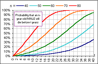
so, for example, females aged n = 60, the probability of dying before age 82 (so t = 22) is
F(60,22) = 1-exp(e^{((60-92.63)/8.78)}(1-e^22/8.78)) = 0.239 or about 24%
and, for males, we get:
F(60,22) = 1-exp(e^{((60-88.18)/10.5)}(1-e^22/10.5)) = 0.385 or about 39%

We use this formula to generate pictures like so:

>Okay, so this is your cumulative distribution, but what about ...?
The density distribution? Here it is (based upon the above estimates):

>No! I was going to ask ... what about annuities?
Yes, let's consider annuities, but first you can play with the formula ...

... and you can compare that estimate chart, above right, with the following:

>Do Canadians live longer?
I'll let you know in a few years ...

>Can't you just change those parameters? Pick another m and c?
Sure, then we can get a good match with the U.S. Dept of Health figures
(shown in light gray).

>But Canadians would die sooner, right?
I'll let you know in a few years ...

Here's a calculator using the parameters which give a better match to the U.S. data:
Another Estimate

Your current Age = years

Enter: 1 of you're female
0 if you're male
How many more years would you like to live = years
Probability of surviving that many years = %

for PART II on annuities.

P.S.

If you'd like to play with an online Excel spreadsheet, click here.