| Distributions: Part III ... continuing from Part II |
In Part I, we assumed that the Variance of a SUM
was equal to the SUM of the Variances and, although that's a good assumption for uncorrelated/independent returns, we were considering
a sum like: z1+z1z2+z1z2z3+...
(where the numbers z are annual Gain Factors like z = eq > 0).
Alas, the terms z1, z1z2, z1z2z3 etc. are NOT uncorrelated (even if the individual gain factors like z1, z2, z3 ARE uncorrelated).
>Is that why your so-called safe withdrawal rates were lousy so high, compared to Monte Carlo?
I think so.
>So, change it!
Okay, but recall (from earlier investigations) our magic formulas for determining the Survival Rate as a function of the Withdrawal Rate:
Assume that our Portfolio is invested in some asset(s) with Mean and Standard Deviation of returns of M and S and
the Inflation Rate is i (so I=1+i is the Inflation Factor) and
g1, g2, g3 are the annual asset Gain Factors (each of the form 1+Return), so that, after n years,
the asset has increased by a factor g1g2...gn (which is then the value of a $1.00 buy-and-hold Portfolio after n years).Starting with a $1.00 portfolio and an initial withdrawal rate of W (increasing with inflation), the value of our portfolio after n withdrawals is
g1g2...gn[1 - W*gMS(n)] where gMS(n) = I/g1 + I2/g1g2 + I3/g1g2g3 + ... + In/g1g2...gn.Hence W*gMS(n) is the reduction factor for a buy-and-hold Portfoio ... reduced by virtue of our withdrawals.
Note that, in order to survive n years, we'll need gMS(n) < 1/W.Let
[a] M = I e-(M - S2/2) the Mean of I / g = (InflationFactor)/(GainFactor)
[b] S2 = M2[eS2-1] the Variance of I / g
[c] Mean = M (1 - Mn) / (1 - M) the Mean of I/g1+I2/g1g2+...+In/g1g2...gn = z1+z1z2+z1z2z3+...+z1z2...zn
[d] SD = ? the Standard Deviation of z1+z1z2+z1z2z3+...+z1z2...zn
Assuming a lognormal distribution of values for gMS(n), we calculate the probability that gMS(n) < 1/W and get the probability that our portfolio will survive n years with an initial withdrawal rate of W, (increasing with inflation), namely N[X] where N is the "standard" normal cumulative distribution function and ... and log is the natural logarithm.
[e] X = log(1/W) - (1/2)log[Mean2/{ 1+SD2 / Mean2 }]
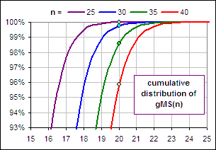
SQRT{log[1+SD2/Mean2]}If, for example, W = 0.05 (meaning a 5% withdrawal rate), then 1/W = 20 and Figure 0 displays typical results (depending upon n, the number of years of withdrawals).
The dots are on the gMS(n) cumulative distribution, evaluated at 1/W = 20.
Figure 0
We want to modify our formula for SD.
Here's what we'll do (reproducing, in part, what we got earlier):
- Assume that the Mean and Standard Deviation of the variables z are M and S (so the Variance is S2, as in [a] and [b], above).
- Then the Mean of z1z2z3...zn is Mn ... that's okay, for independent z-variables
- The Mean of z1 + z1z2 + z1z2z3 + ... + z1z2zn is M + M2 + ... + Mn (giving [c], above) ... that, too, is okay for independent z-variables
- The Variance of z1z2z3...zn is given by (M2+S2)n - M2n ... we got this before and it's also okay for independent z-variables
- BUT, what's SD2, theVariance of z1 + z1z2 + z1z2z3 + ... + z1z2...zn ???
>What did you get before?
We just added the Variances and got SD2 = Σ [(M2+S2)k - M2k]
the sum going from k = 1 to k = n.
>So what's a better formula for that Variance?
Okay. Remember that VAR[x] = (the Average Square) - (the Square of the Average) = Mean[x2] - Mean2[x]
see stat stuff #6.
In particular, we can write:
[1] Mean[x2] = VAR[x] + Mean2[x].
Let's now consider VAR[x+y]. We have (see stat stuff #7):
| VAR[x+y] | = (the Average of (x+y)2) - (the Square of the Average of (x+y)) |
| = VAR[x] + VAR[y] + 2Mean[xy] -2Mean[x]Mean[y] |
If x and y were independent, then Mean[xy] = Mean[x]Mean[y] and we'd get our Variance of a Sum = Sum of Variances.
>You mean VAR[x+y] is NOT equal to VAR[x]+VAR[y]?
Not in our case.
We'll use
[2] VAR[x+y] = VAR[x] + VAR[y] + 2Mean[xy] -2Mean[x]Mean[y]
with x = z1+z1z2+...+z1z2...zk-1 and y = z1z2zk-1...zk.
This x and y ... they aren't independent!
Anyway, that'll give us a prescription for finding VAR[x+y] = VAR[z1 + z1z2 +...+ z1z2...zk-1 + z1z2...zk]
>zzzZZZ
First, notice that the CoVariance of x and y is (see stat stuff #4):
| COVAR[x,y] | = Mean[xy] - Mean[x]Mean[y] |
(See also Pearson Correlation )
Then we can rewrite [2] as:
[3] VAR[x+y] = VAR[x] + VAR[y] + 2COVAR[x,y]
or
[3A] SD2[x+y] = SD2[x] + SD2[y] + 2r SD[x]SD[y]
where r is the Pearson Correlation between x and y.
>Huh? If r = 1 then ... uh ...
Then SD2[x+y]
= SD2[x] + SD2[y] + 2SD[x]SD[y]
= (SD[x] + SD[y])2
so SD[x+y] = SD[x] + SD[y] (as in stat stuff #9).
>The Standard Deviation of a Sum is the Sum of the Standard Deviations?
Yes. Neat, eh? That's for perfect correlation and, if we look at some examples of a thousand uncorrelated random returns
z1, z2, z3 etc. we see that the correlation between z1
and z1z2 and between z1+z1z2 and z1z2z3 etc. etc.
... we find that the Pearson Correlations are very high.
|
>What's "very high"?
Notice that, although the correlation between z1 and z2 is small, the correlation between x = z1+z1z2+...+z1z2...zk-1 and y = z1z2zk-1...zk is about 80%. | 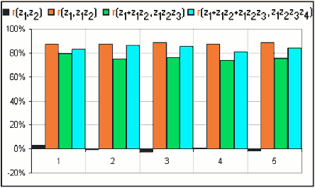 Figure 1 |
|
>So, what's your next attempt at the Standard Deviation of z1+z1z2+z1z2z3+... ?
>Sure, but can't you find an exact result?
>Yeah, yeah. The proof is in the pudding. | 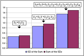 Figure 2 |
SQRT[(M2+S2) - M2] +SQRT[(M2+S2)2 - M4] +SQRT[(M2+S2)3 - M6] +...+SQRT[(M2+S2)n - M2n]
>Can you get a magic formula for that?
I'm thinking, but in the meantime ...
If you recall, from here, we used Variance of Sum = Sum of Variances ... and got :
SD2(gMS(n)) =
SD2(z1 + z1z2 + z1z2z3 + ... +z1z2z3...zn)
=
Σ
(M2+S2)k
- ΣM2k
We even said, at that time: "If we don't like what we get, we'll change it."
>Now you'll change it, eh?
Yes. Now we'll try Standard Deviation of a Sum = Sum of the Standard Deviations.
That would give us:
[4]
SD(gMS(n))
= SQRT[(M2+S2) - M2]
+SQRT[(M2+S2)2 - M4]
+SQRT[(M2+S2)3 - M6]
+...+SQRT[(M2+S2)n - M2n]
We could also write:
[4A]
SD(gMS(n))
= M
SQRT[(1+S2/M2) - 1]
+M2
SQRT[(1+S2/M2)2 - 1]
+...+Mn
SQRT[(1+S2/M2)n - 1].
Let's look (again!) at the relative size of these terms, for
M = 0.09 (that's a 9% return) and S = 0.15 (that's a 15% SD) and I = 1.03 (that's an inflation rate of i = 3%) we get:
M = I e-(M-S2/2) = 0.9520
S2 = I2e-2(M-S2/2)[eS2-1] = 0.0206
|
So M is about 0.95 and 1+S2/M2 is about 1.02 and, if we look at the graph of the SUM 0.95 SQRT[1.02-1]+0.952 SQRT[1.022-1]+0.953 SQRT[1.023-1]+...+0.95n SQRT[1.02n-1], we get Figure 3 which shows the size of the terms ... and their SUM. Our problem is to approximate the SUM graph, for n up to 40 (the number of years of withdrawals) ... as in Figure 4. 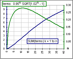 Figure 4 |  Figure 3 |
>Good luck!
Well, since S2/M2
is small, we can approximate (1+S2/M2)k-1
by kS2/M2
... since (1+x)k = 1+kx, for x small.
>For k as large as 40?
Well, not really, but the the proof ...
>Forget the pudding!
|
Anyway, [4A] then becomes:
SD(gMS(n)) = M SQRT[S2/M2] +M2 SQRT[2S2/M2] +...+Mn SQRT[nS2/M2]. or [4B] SD(gMS(n)) = S { 1+M SQRT[2]+M2 SQRT[3]+...+Mn-1SQRT[n] } This gives an approximation which is a mite too small
| 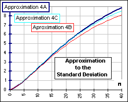 Figure 5 |
You wouldn't happen to recognize the function f(x,n) = 1+21/2x + 31/2x2 + ... +n1/2xn-1
>Are you kidding? Anyway, have you tried using 4A to compare ... uh ...?
To 4C? Yes. Figure 6 gives a comparison of withdrawal / survival rates using Equation 4A, 4B and 4C and, for comparison,
using a Monte Carlo simulation with randomly selected annual returns (from the S&P 500 returns from 1928 to 2000) as well as randomly
selected returns from a normal or lognormal distribution with the same Mean and Standard Deviation. (For the former I used the spreadsheet
described here and, for the latter, I used
the spreadsheet described here.)
|
>An average return of 12.7%?
For the S&P 500? Yes. >And the Monte Carlo stuff? That's the result of 5000 Monte Carlo simulations with the same Mean and SD ... >The S&P curve is crooked. Well, I used 5000 simulations for each withdrawal rate. It'd be smoother if I had used 100,000 simulations and ... >Are you happy?
| 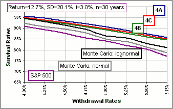 Figure 6 |
>And the Monte Carlo curves don't even agree with the S&P curve!
Yes. The S&P curve uses the actual returns (selected at random, without assuming anything about their distribution) whereas the other
Monte Carlo curves assume a particular distribution.
>I'd say all your approximations are lousy! The proof is in the pudding? Well ...
Yeah. Don't remind me.
But I'm still thinking ...
Okay, let's look (again!) at that magic formula for the Survival Rate, namely N[X] with:
... and "typical" values of Mean and/or SD (as represented by the S&P500) ... to see how that Survival Rate depends upon these parameters. Note that (according to Figure 7) the Survival Rate decreases as Mean or SD increase. Since our formula gives Survival Rates that are too large, we can decrease our calculated Rates by multiplying each of Mean and SD by some number, say C > 1. Then the modified formula becomes:
Since log(1/W) - logC = log(1/CW), this has the effect of changing W to a larger value: CW. For example, if we use [B] instead of [A] (and [4C] to provide a value for SD) with C = 1.20, we get Figure 8 (which we can compare with Figure 6). >You picked your C to get good results, eh?
| 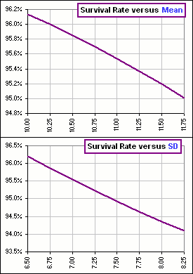 Figure 7 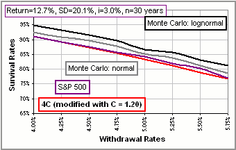 Figure 8 |
>Are you sure that the gMS distribution is lognormal?
Okay. I did a 5000 iteration Monte Carlo simulation, randomly selecting either Lognormal or Normal returns to calculate
gMS(30)
(with 3% inflation) and I got Figure 9 ... which shows a lognormal distribution with the same Mean and Standard Deviation as
gMS(30).
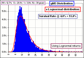
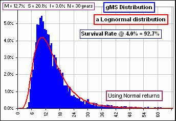
Figure 9
|
>You did 5000 simulations. Is that enough?
>Just what are you plotting?
>So you're happy with that assumption. I mean, assuming that ...
| 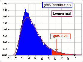 Figure 10 |
>So, is there a spreadsheet?
Uh ... yes, such as it is ... but it's not finished ... I guess. It uses [4B], I think.
However, if you'd like to play, just
RIGHT-click and Save Target here to download
the .ZIPd file.
Recently Walt D. sent me a 1999 paper by
McCabe
who considers survival rates when n = infinity (meaning you live forever).
In particular, McCabe had a slick way of calculating SD for infinite n.
Following McCabe we write:
[5] z1 + z1z2 + z1z2z3 + ...
= z1(1 + z2 + z2z3 + z2z3z4 + ... ) two infinite series
Note that the right side of [5] has the form xy with x = z1 and
y = 1 + z2 + z2z3 + ...
Note, too, that x and y are uncorrelated.
We'll refer to the Mean and Variance of x and y as M[x], M[y] and VAR[x], VAR[y].
For these series, VAR[xy] = VAR[z1 + z1z2 + z1z2z3 + ... ]
is the same as VAR[z2 + z2z3 + z2z3z4 +... ]
'cause they'r the same infinite series when it comes to distributions
is the same as VAR[1 + z2 + z2z3 + + z2z3z4 + ... ] see stat stuff #2
which is VAR[y]. We make a note of this:
[6A] VAR[xy] = VAR[y].
Compare this to:
[6B] VAR[xy] = M2[x]VAR[y] + M2[y]VAR[x] + VAR[x]VAR[y] see stat stuff #10
>I like 6A!
Yes, me too. The simpler version [6A] is a result of the fact that we're dealing with an infinite series
so the distribution of z1 + z1z2 + ... is the same as the distribution of z2 + z2z3 +... 
Proceeding, we put [6A] into [6B] and solve for VAR[xy] = VAR[y] giving the neat result:
[6C] VAR[y] = M2[y]VAR[x] / (1 - M2[x] - VAR[x])
Using the notations in [a], [b], [c] and [d] above:
- M[x] = M[z1] = M the Mean of the terms in gMS
- M[y] = 1+M[z2 + z2z3 + ...] = 1 + Mean note that Mean is the Mean of gMS
- VAR[x] = S2 the Variance of the terms in gMS
- VAR[y] = SD2 the Variance of gMS
| [7] SD2 = |    
1 - M2 - S2 |
so
| [7A] SD2 = |    
1 - M2 eS2 |
|
If we again take our survival rate as N[X], with X defined by [e], namely:
 infinity so that infinity so that
Mean = M (1 - Mn) / (1 - M)  M / (1 - M)
we can compare the survival rates for large values of n (like n = 60) and n = infinity ... as in Figure 11A.
>Is the red curve McCabe's formula.
>Why use [4B]?
>And [4B] is simplest?
>And for larger withdrawal rates?
>So, is there a spreadsheet?
| 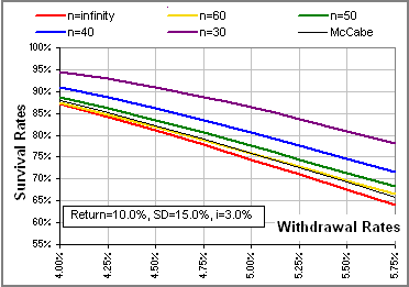 Figure 11A 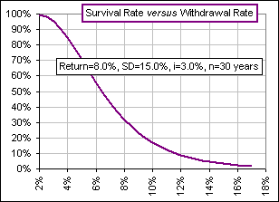 Figure 11B |
 ... don't trust nothin' - yet
  but see more Monte stuff.
