We're considering the following options, starting with a $100 portfolio, then tossing a coin 10 times:

• We can get a guaranteed 5% increase for every toss of the coin: that's 100 (1.05)¹⁰ = $162.89 after 10 tosses.
• We also have the option of getting a 25% gain if we toss a Head and a 10% loss if we toss a Tail. The Expected Value (after 10 tosses) is $206.10 which corresponds to an average 7.5% per toss ... but it's not guaranteed!
• We must decide which is the better option, given our aversion to risk ... and the second option is certainly riskier in the sense that we could lose 10% on every toss and end up with just 100 (0.90)¹⁰ = $34.87.

>Tell me again ... what's that Probability * Value?
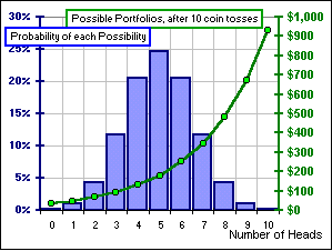
If you performed the 10-toss ritual 1000 times, you'd get, say, 5 Heads, about 25% of the time. (See the left-hand chart, the blue column graph?) That's 25% x 1000 or 250 times. 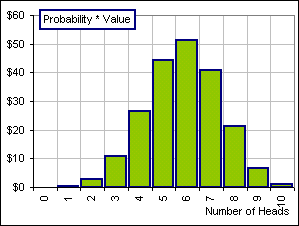That 5-Head outcome would be worth 100 (1.25)⁵(0.90)⁵ = $180.20 so, out of 1000 tries, you'd get 250 of these $180.20 wins, and that's 250 * 180.20 but it takes a thousand tries to get this much so, on average, that's an average of 250 * 180.20 / 1000 = 0.25 * 180.20 (actually, it's about $44), and that's Probability * Value (where 0.25 is the Probability and $180.20 is the Value) and that's shown above in the right-hand chart when Number of Heads is 5 ... see?

Notice that, although the Probability of 5 Heads is larger than the Probability of 6 heads, there's a larger portfolio Value associated with 6 Heads so Probability * Value is actually larger, for 6 Heads ... $51 compared to $44.

>This $44 for 5 heads, and the other possibilities for 0 heads, 1 head ... they all add up to ... uh ...
They all add up to the Expected Value, namly $206.10.

Now we're going to attach a Utility Function which reflects our aversion to risk.

In fact, we're going to multiply Probability x Utility value, not Probability x Dollar value.
(The utility value is sometimes called a utile, but that sounds so much like futile that ...)

>Continue ... please!

1. Suppose the Expected (or probability-weighted Average or Mean) Dollar value is x₀     like the $206.10, mentioned above
2. A given dollar value of $x deviates from this Expected value by an amount x - x₀ .
3. The Utility we attach to this x dollar value is U(x) and we'd like to choose the Utility so it decreases (in some sense^*) for "riskier" distributions.
4. We recall the Taylor Series expansion of U(x) about x = x₀, namely:
   U(x) = U(x₀) + U'(x₀) (x-x₀) + U''(x₀) (x-x₀)²/2 + ...
5. Now, instead of the Expected Value of x, we consider the Expected (or probability-weighted Mean or Average) Value of
   U(x), namely: E[U(x)] = E[U(x₀)] + E[U'(x₀) (x-x₀)] + E[U''(x₀) (x-x₀)²/2] + ...
6. However, the Expected value of a constant, like U(x₀), is equal to that constant and the Expected value of (x-x₀) is zero (because E[x-x₀] = E[x ]-x₀ = x₀-x₀ =0).
7. So we get: E[U(x)] = U(x₀) + U''(x₀) E[(x-x₀)²]/2 + ... and (surprise!) E[(x-x₀)²] is the square of the Standard Deviation of the distribution of x's (the Variance).
8. Our aversion to risk implies that the U(x) curve is concave DOWN and that means the 2nd derivative U''(x₀) is negative so the Expected Value of our utility function (at least in the neighbourhood of the x₀) decreases as the Standard Deviation increases ^* which is what we meant by "in some sense"

>Huh?
We ignore the terms denoted by "+ ..." in (7), above, because they're small when x is close to x₀ and what we get is the equation of a parabola, like Figure 1. The equation in (7) looks like: y = A - B S²/2 which is reminiscent of the relation we used in Part II, between the Annualized and Average return. Remember? It was A = M - S²/2.

>And what does U(x) look like in some other neighbourhood? We use the result in (5) again, but this time we replace x0 by, say, "a" and get: E[U(x)] = E[U(a)] + E[U'(a) (x-a)] + E[U''(a) (x-a)2/2] + ... but now E[(x-a)] is no longer zero (because "a" is a value other than the Mean of x so E[x - a] = E[x ] - a = x0 - a), so the dominant terms give: E[U(x)] = U(a) + U'(a) (x0-a) + ...

Figure 1

and if we assume that U'(x) is positive (which is usually the case, adopting a "more is better" attitude), then the Expected Utility ... that's E[U(x)] ... increases rapidly if the Utility Function increases rapidly (which is the case if U'(x) is larger).

>But you were talking about two options, 5% guaranteed and ...
Ah, yes. So now let's adopt a Utility Function like ..

>Bernoulli's logarithm?
If you insist. So the Expected Value, with a guaranteed 5%, is 100 (1.05)¹⁰ = $162.89 and, using the logarithmic Utility Function, we associate a Utility of log(162.89) = 5.09 whereas, for the +25%/-10% scenario, the Expected Value is 206.10 and the associated Utility is log(206.10) = 5.33 so we've assigned a greater Utility to the latter option.

>I assume you're using log_e. However, aren't you supposed to calculate Expected Utility instead of Utility of Expected Value?
You're quite right. So we look at all the Utility Values, for each possible outcome, and attach a probability to each and sum Probability * Utility and that actually gives 5.19.

In fact, if we simply take the Utility of the Expected Value (as we did, by mistake, above) we'd normally get something larger than if we took the Expected Utility. That's why we got: Utility of Expected Value = U(206.10) = log(206.10) = 5.33 whereas Expected Utility = SUM(Probability * Utility) = 5.19 which is smaller. >We'd normally get something larger? Why "normally"? We'll get to that later, but it happens when the Utility curve is concave DOWN. >Mamma mia! Do I have to remember Expected Value E[x], and Utility Value U(x), and Expected Utility Value E[U(x)], and Utility of Expected Value U(E[x]) and ... Well, maybe it'll get easier as we go along.

Figure 2

>I doubt it. So the Utility we attach to the guaranteed $162.89 is 5.09 and the Utility we attach to the +25%/-10% option is 5.19 so the latter is better, eh?
Yes, if you choose the logarithmic Utility function.
But I think I said (in Part II) that, although U(x) = log(x) was an appropriate Utility Function for Bernoulli's problem, it may not be, for this coin tossing problem. In fact, if something is worthless we'd want to assign a Utility of zero ... and if x = 0, log(x) is hardly 0. Perhaps we should use U(x) = log(1+x) so that U(0) = 0. (This is actually the blue curve in Figure 3, below.)

What we really want is to ...

>Wait! What if I choose the SQRT Utility? What would ...?
For the guaranteed $162.89 you'd get U($162.89) = SQRT(162.89) = 12.8 whereas the Expected Utility (for the +25%/-10% option) is the SUM of Probability * Utility, which turns out to be 13.9 so you'd still choose the +25%/-10% option because you've assigned a Utility Function which gives a greater Expected Utility.

Anyway, as I was saying, what we really want in a Utility Function is ...

>Wait! What if the gain for a Head was, say, 20% instead of 25%?
What Utility function do you choose?
>Uh ... let's say SQRT(x).
Okay. SQRT(162.89) = 12.8 and the Expected utility for a +20%/-10% option is SUM(Probability * Utility) which turns out to be 12.4 so ...
>Aha! Now the guaranteed $162.89 is looking good, eh?

Yes. Now, as I was saying, what we really want in a Utility Function is ...

>Wait! There must be some gain, between 20% and 25%, where ...
Yes. If the gain, for tossing a head, is 21.15% then the Expected Utility for a +21.15%/-10% option is 12.8, the same as the guaranteed Utility, so you'd be indifferent to one or the other. To decide you could ... uh, flip a coin to see what option you'd choose. They have the same Expected Utility, according to the Utility function you've chosen.

Anyway, as I was saying, what we really want in a Utility Function is ...

>Wait! I remember. We want the Utility to decrease as the probability decreases.
Not exactly. Here's what we want:
Suppose $B is 2 times greater than $A, but the probability of winning $B is smaller than the probability of winning $A. Then we'd want to attach a Utility to each of A and B so that U(B) is not 2 times greater than U(A). Increased winnings will increase the Utility, but not in proportion to the value. Even though B/A = 2, maybe U(B) is only 1 1/2 times greater than U(A),
so U(B)/U(A) is only 1 1/2. We'd want U(B)/U(A) to be less than B/A. See?

>So?
So let's see what our utility function might look like:

• Suppose B is greater than A. Then we want
      (1)       U(B) - U(A) > 0     so our Utility function U(x) is increasing ... more is better
• We also want
      (2)       U(B)/U(A) < B/A     so, although x increases from A to B, our Utility function increases by a lesser factor, namely U(B)/U(A).
• We use (1) and (2) to get:
      (3)       0 < (U(B) - U(A)) / (B - A) < U(A)/A
• Now we let B approach A and get, in the limit:
      (4)       0 ≤ U'(A) ≤ U(A)/A

>A picture is worth a thousand ... Here's a picture of our Utility function: where we've imposed the condition from (4), above, namely     0 ≤ U'(x) ≤ U(x) / x In fact, if we set dU/dx = α U(x)/x where α ≤ 1 (which will guarantee that U'(x) ≤ U(x)/x, eh?) then we can solve this differential equation to get U(x) = C xα which, for α = 1/2, gives our SQRT utility and which, in general, you'll remember as a CRRA utility, from Part II, right? >Wrong! Besides, I don't know from nothing about Taylor series and limits and differential equations. Besides, I hate math. Besides, you're a long way from coin tossing. Besides ... Patience. In the meantime, just look at the pictures ...

Figure 3

for Part IV