| How does your Portfolio grow? |
At the end of each year we invest $P, increasing with inflation,
which we assume is I (I = .03 means 3% annual inflation).
We start with a portfolio worth B and we'll track the balance at the end of each year:
After 1 year our portfolio has grown to B(1+R),
and we invest P(1+I).
(See? It's increased ... with inflation!)
Our portfolio is now worth
B(1+R) + P(1+I).
To avoid getting too messy, we'll let
x = (1+R) and
y = (1+I) so, after ONE year (and ONE investment),
our portfolio is worth
Bx + Py
By the end of the second year this portfolio has increased by a factor x = (1+R) to
Bx2 + Pxy and we invest another $P
increased by two years of inflation,
which means we
invest Py2,
giving a portfolio of
Bx2 + P xy + P y2.
There's a magic formula we can use here. It's
x2 + xy + y2
= (x3 - y3)/(x - y)
In order to take advantage of this magic formula, we rewrite
the balance in our portfolio as:
(B - P)x2 + P(x2 + xy + y2)
Using the magic formula, it's (B - P)x2 + P(x3 - y3)/(x - y)
after TWO years and TWO investments.
We jump ahead to the end of the Nth year.
Your portfolio is now
(B - P)xN + P(xN+1 - yN+1)/(x - y)
which can be rewritten as a prettier formula:
| BxN + Py(xN - yN)/(x - y) |
after N years and N investments ... and we've used that magic formula again ... and again!
P.S. If you started with nothing, then, of course, B = 0 and the formula becomes:
| Py(xN - yN)/(x - y) |
| PyN+1 (zN - 1)/(z - 1) where z = x/y |
Note: If you start investing IMMEDIATELY (instead of waiting till the end of the first year), then just replace P by P/y in the above formulas.
If you want to play with this formula, to see how long your portfolio will last (assuming all the parameters remain constant for umpteen years!), then here's a calculator:
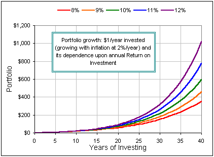
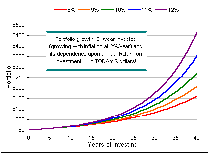
Here's some pretty pictures ...

Investment Assets, after N years

Investment Assets (in today's dollars)
| BxN - Py(xN - yN)/(x - y) |
after N years and N withdrawals. (See Years to Zero.)
... ain't Math wunnerful?
P.S. If'n you'd like to play with your own portfolio, assuming some fixed rate of return and withdrawing an inflation adjusted income, etc., there's a spreadsheet which looks like this:
RIGHT-click on the picture to download a .ZIPd version of the spreadsheet.
Before continuing to the Real World, suppose we retire and start withdrawing a certain percentage of our investment portfolio, say x (where, for a 5% withdrawal rate, we set x = 0.05). Suppose, too, that our withdrawals increase at a fixed rate J due to inflation and that our portfolio also increases at a fixed rate R.
Initially, then, we withdraw $W from a portfolio worth $P and x = W/P is the initial withdrawal rate ... and, after withdrawal, the portfolio is worth $(P-W).
The following year we withdraw $W(1+J) from a portfolio worth $(P-W)(1+R) so the
withdrawal rate is now
W(1+J)/(P-W)(1+R)
which can be written
A (W/P) / { 1 - W/P }
= A x/(1-x)
where A = (1+J)/(1+R)
|
Hence the initial withdrawal rate of x becomes Ax/(1-x) the following year.
We can see this change graphically by plotting
| 
|
For any initial withdrawal rate?
Well, so long as the initial x is greater than
(R-J)/(1+R) which, for 3% inflation and 6% portfolio growth is
(0.06 - 0.03)/(1 + .06) = .028 or 2.8%.
| Random Investment Gains: the real world |
Okay, now let's visit the REAL WORLD, where returns on your investments aren't constant but vary from month to month, sometimes bigger, sometimes smaller, sometimes positive, sometimes NEGATIVE ...
To begin, we assume we've got a $100K portfolio and we just sit and watch it grow. We also suppose that our Rate of Return averages 10% but varies month to month from, say, -30% to maybe +50% or maybe ... (Of course, if the annual Rate of Return is +50% that'd be a monthly Return of 1.51/12 - 1 or 3.4% per month.)
In fact, here's a picture of a typical collection of 120 Rates of Return over a ten year period.
Of course, when we say Rate of Return we mean the annual Rate (even tho' these rates
get applied as the eqivalent monthly rate). Anyway, you see that most are around 10% (that's the average rate)
but there are also a few at -30% and at +50% and other rates in between.
Our one big question is:
|
 Fig. 1 |
 Fig. 2 |
Well, that's more than one big question, but you get the idea. Here's a typical portfolio, with randomly distributed Rates of Return as illustrated above. Not exactly the smooooth curve we saw earlier. Indeed, if we got 10% per year for ten years our final portfolio would be worth about $259K, not $207K as illustrated. Of course, who knows, maybe we're lucky and the random selection of Rates of Return might give a bunch somewhat larger than 10% ... but, we shouldn't count on it. In fact, even though we might insist that our set of Returns (for the 120 months) all have a specified mean ... and a specified "spread" about this mean (or volatility: see SD-stuff) ... there are still an infinite number of Returns with these properties! |
|
Further, once we pick a set, the order in which we apply these Returns to
our portfolio will affect the outcome. Hence, to get some idea of the possible outcomes,
we must consider lots of examples. Okay, suppose we consider a few dozen such examples (36 to be exact). The possible final portfolios could be distributed as illustrated in Fig. 3, where we randomly generated three dozen sets of Returns (but each distributed about 10% as in Fig. 1). Notice that most gains do run around 10% ... but one portfolio had a gain of nearly 20% (and, alas, yet another was down about 0.5%). |
 Fig. 3 |
Anyway, here are pictures for a possible, typical portfolio and a possible distribution of final values, for 36 portfolios:


Sad to say, one of the 36 portfolios actually went bust. Of course, if we withdrew, say 6% annually (instead of 9%) and invested in stocks/funds with less volatility, we could get this picture(s):


In the leftmost picture, note that the spread of Returns is less, meaning less volatility (though a few are negative). In fact, for the earlier case, the volatility was 20% (as measured by the Standard Deviation of the 120 Rates) and here we've changed the volatility to 10%. Note, too, that most of the 36 portfolios increased after ten years and none went broke ... but we can't guarantee that! Indeed, there are two effects at work here:
- The Mean and Volatility of the investment Returns (which characterize the statistical distribution)
- The particular sequence of Returns selected (from that distribution of Returns)
| It's sort of like throwing a single die, with numbers "1" to "6" on each side. There are six possible outcomes and each is equally probable. Now consider a die with 1000 sides. On each side there is written a number (representing a Rate of Return percentage), but some numbers appear on several sides. In fact, if we plot the number of occurrences of the various percentages, we'd get a chart like Fig. 4 where the most common numbers are around 10% but there are a few out near the edges at -30% and +50%. This chart gives the statistical distribution of numbers on the 1000 sides, characterized by their Mean and Standard Deviation (or Volatility). It's effect #1 in the collection of effects identified above ... and we haven't even tossed the die yet! |
 Fig. 4 |
- yield the same number, say +50%

- be skewed toward the negative numbers

- be nicely distributed according the specified Mean and Volatility
To get a feel for the variation in outcomes (in our portfolio, after ten years) we need to consider lots of examples ... lots of people throwing the die 120 times ... like mebbe 36 people and their 36 portfolios? (That's what we did above, in Fig. 3. Remember?)
The easy part is the accumulation of assets. We make monthly contributions to our investment portfolio till it hurts. Then comes the hard part: the eventual withdrawal phase when we must withdraw a monthly amount to pay for our living expenses. What most people fear is going broke at age 80 say (when they can't even qualify for a job at McDonalds). How do we know what is a safe withdrawal rate ... where we don't outlive our assets? An important question that does not have a simple answer. The answer involves uncertainty and dealing with probabilities, as we've seen.
Of course, the above stuff assumes the future evolves as the past (using volatility and mean returns, etc. over the past umpteen years). What would have happened had we invested in, say, the S&P 500 over the past fifty years, withdrawing each month a certain percentage of a $100K portfolio. (We withdraw monthly, but the monthly amount increases each year with inflation.) Our portfolio would have looked like so:

(or, if we don't increase our withdrawals ...

SO ... 6 1/2% withdrawal rate looks pretty safe, eh? BUT, why begin in January, 1950? What about Jan/55 or June/76 or ... ? Would that have made a difference?


 You start with $100K at the date indicated, investing in the S&P 500 for 20 years,
withdrawing an annual (2%-inflation-adjusted) 6.5% Mamma mia!
 The twenty years, starting in the Jan/65, looks pretty scary. So what withdrawal rate would have been safer?

Your portfolio, starting with $100K on Jan 1, 1965 (investing in the S&P 500 for 20 years) and withdrawing an annual (2%-inflation-adjusted) 4% or 5% or 6%
So, how often would a 20-year investment in the S&P 500 be reduced to zero if we just withdrew 5% or 6% or ... and we did NOT increase the withdrawal with inflation. If we consider the 360 20-years periods lying in the range Jan, 1950 to Jan, 2000 (that's thirty years worth), this is what we'd get:

How often would your portfolio have gone to zero, (investing in the S&P 500 for 20 years) with a FIXED annual withdrawal rate (NOT inflation-adjusted).
|
 for Safe Withdrawal Rates for Safe Withdrawal Rates
|  for Optimal Withdrawal Rates for Optimal Withdrawal Rates
|
Oh ... one other thing: you can take a peek at Random Walks which also involves predicting the future by examining the past ... sort of.
Then, too, you may want to check out Saving for Retirement.

